Classification: linear and logistic regression

 As the amount of available data, the strength of computing power, and the number of algorithmic improvements continue to rise, so does the importance of data science and machine learning. Classification is among the most important areas of machine learning, and logistic regression is one of its basic methods. By the end of this tutorial, you’ll have learned about classification in general and the fundamentals of logistic regression in particular, as well as how to implement logistic regression in Python.

In this tutorial, you’ll learn:

• What linear and logistic regression is
• What linear and logistic regression is used for
• How linear and logistic regression works
• How to implement linear and logistic regression in Python, step by step

Linear Equations

A linear equation is an equation for a straight line

These are all linear equations:

		y = 2x + 1
		5x = 6 + 3y
		y/2 = 3 − x

Let us look more closely at one example:

Example: y = 2x + 1 is a linear equation:

The graph of y = 2x+1 is a straight line

 

• When x increases, y increases twice as fast, so we need 2x
• When x is 0, y is already 1. So +1 is also needed
• And so: y = 2x + 1

Here are some example values:

x	y = 2x + 1
-1	y = 2 × (-1) + 1 = -1
0	y = 2 × 0 + 1 = 1
1	y = 2 × 1 + 1 = 3
2	y = 2 × 2 + 1 = 5

Check for yourself that those points are part of the line above!

Different Forms

There are many ways of writing linear equations, but they usually have constants (like "2" or "c") and must have simple variables (like "x" or "y").

Examples: These are linear equations:

		y = 3x − 6
		y − 2 = 3(x + 1)
		y + 2x − 2 = 0
		5x = 6
		y/2 = 3

But the variables (like "x" or "y") in Linear Equations do NOT have:

• Exponents (like the 2 in x²)
• Square roots, cube roots, etc

Examples: These are NOT linear equations:

		y2 − 2 = 0
		3√x − y = 6
		x3/2 = 16

Slope-Intercept Form

The most common form is the slope-intercept equation of a straight line:

Slope (or Gradient)	Y Intercept

Example: y = 2x + 1

• Slope: m = 2
• Intercept: b = 1

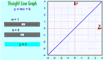Play With It ! You can see the effect of different values of m and b at Explore the Straight Line Graph

Point-Slope Form

Another common one is the Point-Slope Form of the equation of a straight line:

y − y1 = m(x − x1)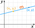

Example: y − 3 = (¼)(x − 2)

It is in the form y − y₁ = m(x − x₁) where:

• y₁ = 3
• m = ¼
• x₁ = 2

General Form

And there is also the General Form of the equation of a straight line:

Ax + By + C = 0

(A and B cannot both be 0)

Example: 3x + 2y − 4 = 0

It is in the form Ax + By + C = 0 where:

• A = 3
• B = 2
• C = −4

There are other, less common forms as well.

As a Function

Sometimes a linear equation is written as a function, with f(x) instead of y:

y = 2x − 3

f(x) = 2x − 3

These are the same!

And functions are not always written using f(x):

y = 2x − 3

w(u) = 2u − 3

h(z) = 2z − 3

These are also the same!

The Identity Function

There is a special linear function called the "Identity Function":

f(x) = x

And here is its graph:

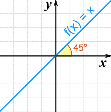
It makes a 45° (its slope is 1)

It is called "Identity" because what comes out is identical to what goes in:

In	Out
0	0
5	5
−2	−2
...etc	...etc

Constant Functions

Another special type of linear function is the Constant Function ... it is a horizontal line:

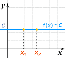
f(x) = C

No matter what value of "x", f(x) is always equal to some constant value.

Least Squares Regression

Line of Best Fit

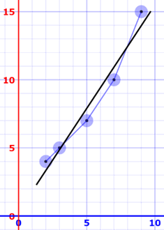
Imagine you have some points, and want to have a line that best fits them like this:

We can place the line "by eye": try to have the line as close as possible to all points, and a similar number of points above and below the line.

But for better accuracy let's see how to calculate the line using Least Squares Regression.

The Line

Our aim is to calculate the values m (slope) and b (y-intercept) in the equation of a line :

y = mx + b

Where:

• y = how far up
• x = how far along
• m = Slope or Gradient (how steep the line is)
• b = the Y Intercept (where the line crosses the Y axis)

Steps

To find the line of best fit for N points:

Step 1: For each (x,y) point calculate x² and xy

Step 2: Sum all x, y, x² and xy, which gives us Σx, Σy, Σx² and Σxy (Σ means "sum up")

Step 3: Calculate Slope m:

m = N Σ(xy) − Σx ΣyN Σ(x²) − (Σx)²

(N is the number of points.)

Step 4: Calculate Intercept b:

b = Σy − m ΣxN

Step 5: Assemble the equation of a line

y = mx + b

Done!

Example

Let's have an example to see how to do it!

Example: Sam found how many hours of sunshine vs how many ice creams were sold at the shop from Monday to Friday:

"x" Hours of Sunshine	"y" Ice Creams Sold
2	4
3	5
5	7
7	10
9	15

Let us find the best m (slope) and b (y-intercept) that suits that data

y = mx + b

 

Step 1: For each (x,y) calculate x² and xy:

x	y	x2	xy
2	4	4	8
3	5	9	15
5	7	25	35
7	10	49	70
9	15	81	135

Step 2: Sum x, y, x² and xy (gives us Σx, Σy, Σx² and Σxy):

x	y	x2	xy
2	4	4	8
3	5	9	15
5	7	25	35
7	10	49	70
9	15	81	135
Σx: 26	Σy: 41	Σx2: 168	Σxy: 263

Also N (number of data values) = 5

Step 3: Calculate Slope m:

m = N Σ(xy) − Σx ΣyN Σ(x²) − (Σx)²

= 5 x 263 − 26 x 415 x 168 − 26²

= 1315 − 1066840 − 676

= 249164 = 1.5183...

Step 4: Calculate Intercept b:

b = Σy − m ΣxN

= 41 − 1.5183 x 265

= 0.3049...

Step 5: Assemble the equation of a line:

y = mx + b

y = 1.518x + 0.305

Let's see how it works out:

x	y	y = 1.518x + 0.305	error
2	4	3.34	−0.66
3	5	4.86	−0.14
5	7	7.89	0.89
7	10	10.93	0.93
9	15	13.97	−1.03

Here are the (x,y) points and the line y = 1.518x + 0.305 on a graph:

Nice fit!

Sam hears the weather forecast which says "we expect 8 hours of sun tomorrow", so he uses the above equation to estimate that he will sell

y = 1.518 x 8 + 0.305 = 12.45 Ice Creams

Sam makes fresh waffle cone mixture for 14 ice creams just in case. Yum.

How does it work?

It works by making the total of the square of the errors as small as possible (that is why it is called "least squares"):

The straight line minimizes the sum of squared errors

So, when we square each of those errors and add them all up, the total is as small as possible.

You can imagine (but not accurately) each data point connected to a straight bar by springs:

Boing!

Outliers

Be careful! Least squares is sensitive to outliers. A strange value will pull the line towards it.

Linear Regression Example in Python

The example below uses only the first feature of the diabetes dataset, in order to illustrate the data points within the two-dimensional plot. The straight line can be seen in the plot, showing how linear regression attempts to draw a straight line that will best minimize the residual sum of squares between the observed responses in the dataset, and the responses predicted by the linear approximation.

The coefficients, residual sum of squares and the coefficient of determination are also calculated.

Out:

Coefficients:
 [938.23786125]
Mean squared error: 2548.07
Coefficient of determination: 0.47

# Code source: Jaques Grobler
# License: BSD 3 clause

import matplotlib.pyplot as plt
import numpy as np
from sklearn import datasets, linear_model
from sklearn.metrics import mean_squared_error, r2_score

# Load the diabetes dataset
diabetes_X, diabetes_y = datasets.load_diabetes(return_X_y=True)

# Use only one feature
diabetes_X = diabetes_X[:, np.newaxis, 2]

# Split the data into training/testing sets
diabetes_X_train = diabetes_X[:-20]
diabetes_X_test = diabetes_X[-20:]

# Split the targets into training/testing sets
diabetes_y_train = diabetes_y[:-20]
diabetes_y_test = diabetes_y[-20:]

# Create linear regression object
regr = linear_model.LinearRegression()

# Train the model using the training sets
regr.fit(diabetes_X_train, diabetes_y_train)

# Make predictions using the testing set
diabetes_y_pred = regr.predict(diabetes_X_test)

# The coefficients
print("Coefficients: \n", regr.coef_)
# The mean squared error
print("Mean squared error: %.2f" % mean_squared_error(diabetes_y_test, diabetes_y_pred))
# The coefficient of determination: 1 is perfect prediction
print("Coefficient of determination: %.2f" % r2_score(diabetes_y_test, diabetes_y_pred))

# Plot outputs
plt.scatter(diabetes_X_test, diabetes_y_test, color="black")
plt.plot(diabetes_X_test, diabetes_y_pred, color="blue", linewidth=3)

plt.xticks(())
plt.yticks(())

plt.show()

Total running time of the script: ( 0 minutes 0.061 seconds)

Introduction to Linear Regression in Python

A quick tutorial on how to implement linear regressions with the Python statsmodels & scikit-learn libraries.

Example linear regression model using simulated data

Linear regression is a basic predictive analytics technique that uses historical data to predict an output variable. It is popular for predictive modelling because it is easily understood and can be explained using plain English.

Linear regression models have many real-world applications in an array of industries such as economics (e.g. predicting growth), business (e.g. predicting product sales, employee performance), social science (e.g. predicting political leanings from gender or race), healthcare (e.g. predicting blood pressure levels from weight, disease onset from biological factors), and more.

Understanding how to implement linear regression models can unearth stories in data to solve important problems. We’ll use Python as it is a robust tool to handle, process, and model data. It has an array of packages for linear regression modelling.

The basic idea is that if we can fit a linear regression model to observed data, we can then use the model to predict any future values. For example, let’s assume that we have found from historical data that the price (P) of a house is linearly dependent upon its size (S) — in fact, we found that a house’s price is exactly 90 times its size. The equation will look like this:

P = 90*S

With this model, we can then predict the cost of any house. If we have a house that is 1,500 square feet, we can calculate its price to be:

P = 90*1500 = $135,000

In this blog post, we cover:

1. The basic concepts and mathematics behind the model
2. How to implement linear regression from scratch using simulated data
3. How to implement linear regression using statsmodels
4. How to implement linear regression using scikit-learn

This brief tutorial is adapted from the Next XYZ Linear Regression with Python course, which includes an in-browser sandboxed environment, tasks to complete, and projects using public datasets.

Basic concepts and mathematics

There are two kinds of variables in a linear regression model:

• The input or predictor variable is the variable(s) that help predict the value of the output variable. It is commonly referred to as X.
• The output variable is the variable that we want to predict. It is commonly referred to as Y.

To estimate Y using linear regression, we assume the equation:

Yₑ = α + β X

where Yₑ is the estimated or predicted value of Y based on our linear equation.

Our goal is to find statistically significant values of the parameters α and β that minimise the difference between Y and Yₑ.

If we are able to determine the optimum values of these two parameters, then we will have the line of best fit that we can use to predict the values of Y, given the value of X.

So, how do we estimate α and β? We can use a method called ordinary least squares.

Ordinary Least Squares

Green lines show the difference between actual values Y and estimate values Yₑ

The objective of the least squares method is to find values of α and β that minimise the sum of the squared difference between Y and Yₑ. We will not go through the derivation here, but using calculus we can show that the values of the unknown parameters are as follows:

where X̄ is the mean of X values and Ȳ is the mean of Y values.

If you are familiar with statistics, you may recognise β as simply
Cov(X, Y) / Var(X).

Linear Regression From Scratch

In this post, we’ll use two Python modules:

• statsmodels — a module that provides classes and functions for the estimation of many different statistical models, as well as for conducting statistical tests, and statistical data exploration.
• scikit-learn — a module that provides simple and efficient tools for data mining and data analysis.

Before we dive in, it is useful to understand how to implement the model from scratch. Knowing how the packages work behind the scenes is important so you are not just blindly implementing the models.

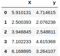
To get started, let’s simulate some data and look at how the predicted values (Yₑ) differ from the actual value (Y):

import pandas as pd
import numpy as np
from matplotlib import pyplot as plt

# Generate 'random' data
np.random.seed(0)
X = 2.5 * np.random.randn(100) + 1.5   # Array of 100 values with mean = 1.5, stddev = 2.5
res = 0.5 * np.random.randn(100)       # Generate 100 residual terms
y = 2 + 0.3 * X + res                  # Actual values of Y

# Create pandas dataframe to store our X and y values
df = pd.DataFrame(
    {'X': X,
     'y': y}
)

# Show the first five rows of our dataframe
df.head()

If the above code is run (e.g. in a Jupyter notebook), this would output something like:

To estimate y using the OLS method, we need to calculate xmean and ymean, the covariance of X and y (xycov), and the variance of X (xvar) before we can determine the values for alpha and beta.

# Calculate the mean of X and y
xmean = np.mean(X)
ymean = np.mean(y)

# Calculate the terms needed for the numator and denominator of beta
df['xycov'] = (df['X'] - xmean) * (df['y'] - ymean)
df['xvar'] = (df['X'] - xmean)**2

# Calculate beta and alpha
beta = df['xycov'].sum() / df['xvar'].sum()
alpha = ymean - (beta * xmean)
print(f'alpha = {alpha}')
print(f'beta = {beta}')

Out:
alpha = 2.0031670124623426
beta = 0.32293968670927636

Great, we now have an estimate for alpha and beta! Our model can be written as Yₑ = 2.003 + 0.323 X,​ and we can make predictions:

ypred = alpha + beta * X

Out:
array([3.91178282, 2.81064315, 3.27775989, 4.29675991, 3.99534802,
       1.69857201, 3.25462968, 2.36537842, 2.40424288, 2.81907292,
       ...
       2.16207195, 3.47451661, 2.65572718, 3.2760653 , 2.77528867,
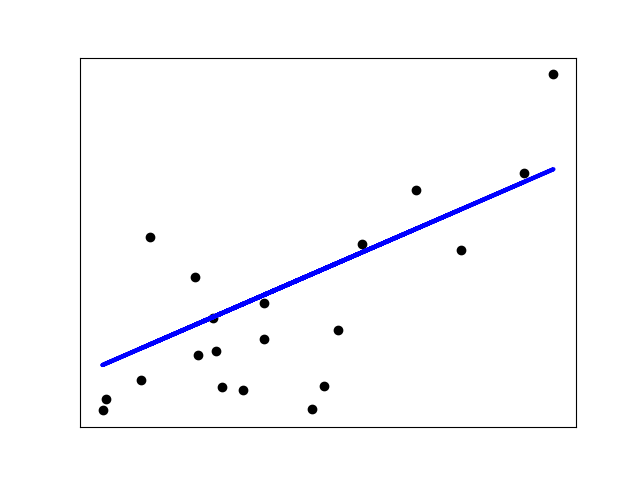
       3.05802784, 2.49605373, 3.92939769, 2.59003892, 2.81212234])

Let’s plot our prediction ypred against the actual values of y, to get a better visual understanding of our model.

# Plot regression against actual data
plt.figure(figsize=(12, 6))
plt.plot(X, ypred)     # regression line
plt.plot(X, y, 'ro')   # scatter plot showing actual data
plt.title('Actual vs Predicted')
plt.xlabel('X')
plt.ylabel('y')

plt.show()

The blue line is our line of best fit, Yₑ = 2.003 + 0.323 X. We can see from this graph that there is a positive linear relationship between X and y. Using our model, we can predict y from any values of X!

For example, if we had a value X = 10, we can predict that:
Yₑ = 2.003 + 0.323 (10) = 5.233.

Linear Regression with statsmodels

Now that we have learned how to implement a linear regression model from scratch, we will discuss how to use the ols method in the statsmodels library.

To demonstrate this method, we will be using a very popular advertising dataset about various costs incurred on advertising by different mediums and the sales for a particular product. You can download this dataset here.

We will only be looking at the TV variable in this example — we will explore whether TV advertising spending can predict the number of sales for the product. Let’s start by importing this csv file as a pandas dataframe using read_csv():

# Import and display first five rows of advertising dataset
advert = pd.read_csv('advertising.csv')
advert.head()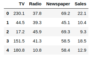

First, we use statsmodels’ ols function to initialise our simple linear regression model. This takes the formula y ~ X, where X is the predictor variable (TV advertising costs) and y is the output variable (Sales). Then, we fit the model by calling the OLS object’s fit() method.

import statsmodels.formula.api as smf

# Initialise and fit linear regression model using `statsmodels`
model = smf.ols('Sales ~ TV', data=advert)
model = model.fit()

We no longer have to calculate alpha and beta ourselves as this method does it automatically for us! Calling model.params will show us the model’s parameters:

Out:
Intercept    7.032594
TV           0.047537
dtype: float64

In the notation that we have been using, α is the intercept and β is the slope i.e. α = 7.032 and β = 0.047.

Thus, the equation for the model will be: Sales = 7.032 + 0.047*TV

In plain English, this means that, on average, if we spent $100 on TV advertising, we should expect to sell 11.73 units.

Now that we’ve fit a simple regression model, we can try to predict the values of sales based on the equation we just derived using the .predict method.

We can also visualise our regression model by plotting sales_pred against the TV advertising costs to find the line of best fit:

# Predict values
sales_pred = model.predict()

# Plot regression against actual data
plt.figure(figsize=(12, 6))
plt.plot(advert['TV'], advert['Sales'], 'o')           # scatter plot showing actual data
plt.plot(advert['TV'], sales_pred, 'r', linewidth=2)   # regression line
plt.xlabel('TV Advertising Costs')
plt.ylabel('Sales')
plt.title('TV vs Sales')

plt.show()

We can see that there is a positive linear relationship between TV advertising costs and Sales — in other words, spending more on TV advertising predicts a higher number of sales!

With this model, we can predict sales from any amount spent on TV advertising. For example, if we increase TV advertising costs to $400, we can predict that sales will increase to 26 units:

new_X = 400
model.predict({"TV": new_X})

Out:
0    26.04725
dtype: float64

Linear Regression with scikit-learn

We’ve learnt to implement linear regression models using statsmodels…now let’s learn to do it using scikit-learn!

For this model, we will continue to use the advertising dataset but this time we will use two predictor variables to create a multiple linear regression model. This is simply a linear regression model with more than one predictor, and is modelled by:

Yₑ = α + β₁X₁ + β₂X₂ + … + βₚXₚ, where p is the number of predictors.

In our example, we will be predicting Sales using the variables TV and Radio i.e. our model can be written as:

Sales = α + β₁*TV + β₂*Radio.

First, we initialise our linear regression model, then fit the model to our predictors and output variables:

from sklearn.linear_model import LinearRegression

# Build linear regression model using TV and Radio as predictors
# Split data into predictors X and output Y
predictors = ['TV', 'Radio']
X = advert[predictors]
y = advert['Sales']

# Initialise and fit model
lm = LinearRegression()
model = lm.fit(X, y)

Again, there is no need to calculate the values for alpha and betas ourselves – we just have to call .intercept_ for alpha, and .coef_ for an array with our coefficients beta1 and beta2:

print(f'alpha = {model.intercept_}')
print(f'betas = {model.coef_}')

Out:
alpha = 2.921099912405138
betas = [0.04575482 0.18799423]

Therefore, our model can be written as:

Sales = 2.921 + 0.046*TV + 0.1880*Radio.

We can predict values by simply using .predict():

model.predict(X)

Out:
array([20.555464, 12.345362, 12.337017, 17.617115, 13.223908,
       12.512084, 11.718212, 12.105515,  3.709379, 12.551696,
       ...
       12.454977,  8.405926,  4.478859, 18.448760, 16.4631902,
        5.364512,  8.152375, 12.768048, 23.792922, 15.15754285])

Now that we’ve fit a multiple linear regression model to our data, we can predict sales from any combination of TV and Radio advertising costs! For example, if we wanted to know how many sales we would make if we invested $300 in TV advertising and $200 in Radio advertising…all we have to do is plug in the values!

Out:
[54.24638977]

This means that if we spend $300 on TV advertising and $200 on Radio advertising, we should expect to see, on average, 54 units sold.

We covered how to implement linear regression from scratch and by using statsmodels and scikit-learn in Python. In practice, you will have to know how to validate your model and measure efficacy, how to select significant variables for your model, how to handle categorical variables, and when and how to perform non-linear transformations.